| 4C0d-2 | Actinobacteria | Alphaproteobacteria | |
|---|---|---|---|
| Feces | 211574 | 155830 | 35987 |
| Freshwater | 173 | 996508 | 23428 |
| Freshwater (creek) | 66 | 17426 | 6472 |
| Mock | 48 | 268678 | 392 |
| Ocean | 29 | 193931 | 385934 |
| Sediment (estuary) | 19 | 2018 | 377 |
| Skin | 18 | 10683 | 397 |
| Soil | 102 | 763 | 28398 |
| Tongue | 60 | 101237 | 1323 |
1. Introduction
The microbiome is the collection of microorganisms that live together in a particular place (e.g. river, soil, skin, gut,etc). With modern technologies we can identify thousands of different microbial species in a sample. These technologies give counts for all of these species. These counts, however, cannot be directly interpreted as a count of the absolute abundance of that species in the sample. These counts should be interpreted relatively to the total count in the sample.
Microbiome data typically contains counts for thousands of microbial species, but for this project, 182 most abundant species were selected. Each microbial species has an official Latin name according to a taxonomy. At the lowest level these organisms can be identified to species level, which are combined into genera, which are in turn combined into families. This is followed by order, class, division, and phylum. For this report, the classification of the 182 species into Phylum and Class was studied.
We explored the relationship between microbial composition and the sample type using correspondence analysis (CA), which based on singular value decomposition (SVD) method. More specifically, we aimed to identify which microbial species are more present in certain sample types and if there are any common microbial compositions between different taxonomic classifications.
2. Research Question
What is the Relationship between the microbial composition and the sample type?
3. Methodology
3.1 Data Exploration
The microbiome data-set provided absolute counts of 182 species in 26 samples taken from Caporaso et.al. (2011) illustrated in the (\(182\) x \(26\)) GP.OTU data matrix. The microbial species had official Latin names with the considered taxonomic order classifying the 182 microbial species into phylum and class, illustrated in the GP.Tax data. The GP.Sample data gave information about sample types, of which some had a non-human while some human origin.
Although performance of principal component analysis on the original OTU data matrix could have detailed the relationship of the microbial species at sample type level, visualization and interpretation would be limited due to huge dimensions and lack of taxonomy information. Therefore we transformed the original data to two compressed matrices to include phylum-sample type levels and class-sample type levels. The first matrix was a contingency table with 9 sample types in the rows and 5 phyla in the columns, for the second matrix we had a distribution of 16 bacteria classes over 9 sample types.The two matrices are shown in table 1 and table 2 below:
| Actinobacteria | Bacteroidetes | Cyanobacteria | |
|---|---|---|---|
| Feces | 155830 | 2257645 | 214794 |
| Freshwater | 996508 | 217191 | 1082952 |
| Freshwater (creek) | 17426 | 68749 | 3208029 |
| Mock | 268678 | 783031 | 5286 |
| Ocean | 193931 | 877997 | 484923 |
| Sediment (estuary) | 2018 | 5259 | 13982 |
| Skin | 10683 | 10452 | 28586 |
| Soil | 763 | 4989 | 2579 |
| Tongue | 101237 | 142264 | 17600 |
We shall therefore use these two compressed data sets to perform correspondence analysis.
3.2 Correspondence Analysis
In this section, we describe how the correspondence analysis is carried out. For a matrix X with dimensions \(M \times N\) which is a contingency table, the procedure for the correspondence analysis is described below:
First, the total counts of each category are needed. For this the row and column marginal totals are calculated: \[ x_{m.} = \sum_{n=1}^N x_{mn},\hspace{2cm} x_{.n} = \sum_{m=1}^M x_{mn}\]
Next, the total count is calculated from the marginal totals: \[ T = \sum_{m=1}^M x_{m.} = \sum_{n=1}^N x_{.n}\] In a next step, the marginal probabilities are computed.
\[f_{m.}=\frac{x_{m.}}{T},\hspace{2cm}f_{.n}=\frac{x_{.n}}{T}\] The total count is then used to compute the expected frequencies for each cell:
\[ E_{mn}=T.f_{m.}f_{.n}\] Now, a chi squared test is preformed using the following formula:
\[\chi^2=\sum_{m, n} \frac{(x_{mn}-E_{mn})^2}{E_{mn}}\]
The chi square test is used to test if there is an association between the rows and the columns of the data. If there is a statistical significant association, we will perform correspondence analysis using Singular Value Decomposition method.
First, we develop a proportion matrix by dividing X by its sum T:
\[P=\frac{X}{T}\] We compute row and column weights by: \[F_M=(f_{1.}, f_{2.},.., f_{M.}),\hspace{2cm}F_N=(f_{.1}, f_{.2},.., f_{.N})\] The weights are then transformed into diagonal matrices: \[W_m = diag(1/\sqrt(F_M)),\hspace{2cm}W_n = diag(1/\sqrt(F_N))\] The B matrix is given by:
\[B = W_m(P- (F_M)^t F_N)W_n\]
The method of Singular Value Decomposition is performed for B, which is an M x N matrix with rank M.
Using this notation, we derive the SVD of B as: \[B = U \times S \times V^t\]
where:
- \(U\) is a \(M \times M\) matrix of left singular vectors. The left singular vectors in U represent the relationship between the M sample origins and the M dimensions.
- \(S\) is a \(M \times M\) diagonal matrix of singular values. The diagonal matrix S represents the variance explained by the M dimensions.
- \(V\) is a \(N \times M\) matrix of right singular vectors. The right singular vectors in V represent the relationship between the N taxonomic classifications and M dimensions.
After this the correspondence analysis is carried out. Now a choice must be made in terms of dimension reduction. This choice is based on the eigenvalues from the correspondence analysis because they indicate the amount of variance explained in the solution. Once this is done, biplots are used to visualize the relationships between sample origins and taxonomic classifications. The coordinates are used to interpret the contributions and lastly the contribution of row and column profiles can be explained as they indicate the importance of each category to each dimension.
3.3 Model Assessment
3.3.1 Test for dependence
For our contingency tables, we used the Chi-square test to evaluate whether there is a significant dependence between row and column categories. Although we found that the row and column variables were statistically significant with associated (p-value < 0.0001), the chi-square test does not provide detailed information for such relationship. The correspondence analysis, which is based on similar mathematical formula, can be used to investigate this association by biplots and coordinates interpretation.
3.3.2 Variability between dimensions
Eigenvalues correspond to the amount of information retained by each dimension, specifically, the variances it explains. The higher the retention, the more subtlety in the original data is retained in the low-dimensional solution (M. Bendixen 2003). In the scree plot below the dimensions are illustrated in descending order based on their eigenvalues.
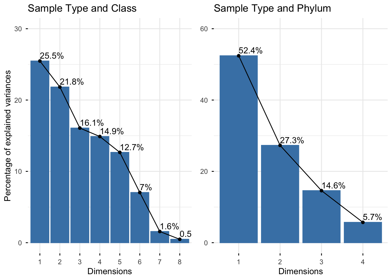
The first scree plot shows that dimension 1 explains the largest amount of variance (25.5%), followed by dimension 2 (21.8%), and so on. However, our analysis reveals that the first two dimensions only account for 47.29% of the total variation or inertia.
In contrast, the second scree plot suggests that dimension 1 performs better, explaining as much as 52.4% of the total variance. Dimension 2 also conveys a substantial figure of 27.3%. Together, these two dimensions account for a total of 79.9% of the variation.
Notably in our first matrix compared to our second matrix, the number of classes exceeds the number of phyla, resulting in a higher-dimensional class matrix. Consequently, reducing the column dimensions of these matrices to 2 diminishes the performance of the first two dimensions, with only 47.29% of the total variation explained, compared to 79.9% when using the higher-dimensional matrices.
4. Results
4.1 Row Profile Interpretation
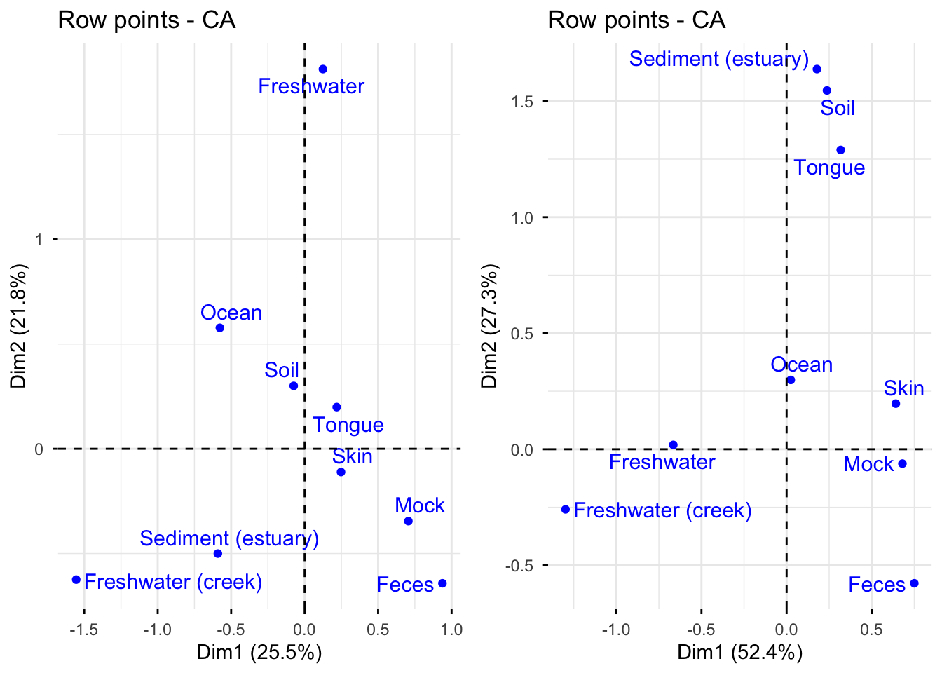
As can be seen from the first plot, the first dimension is mostly determined by freshwater (creek) while the second dimension is determined by freshwater.
The second plot shows that freshwater (creek) best describes the first dimension and sediment (estuary) is the best indicator of the second dimension.
4.2 Column Profile Interpretation
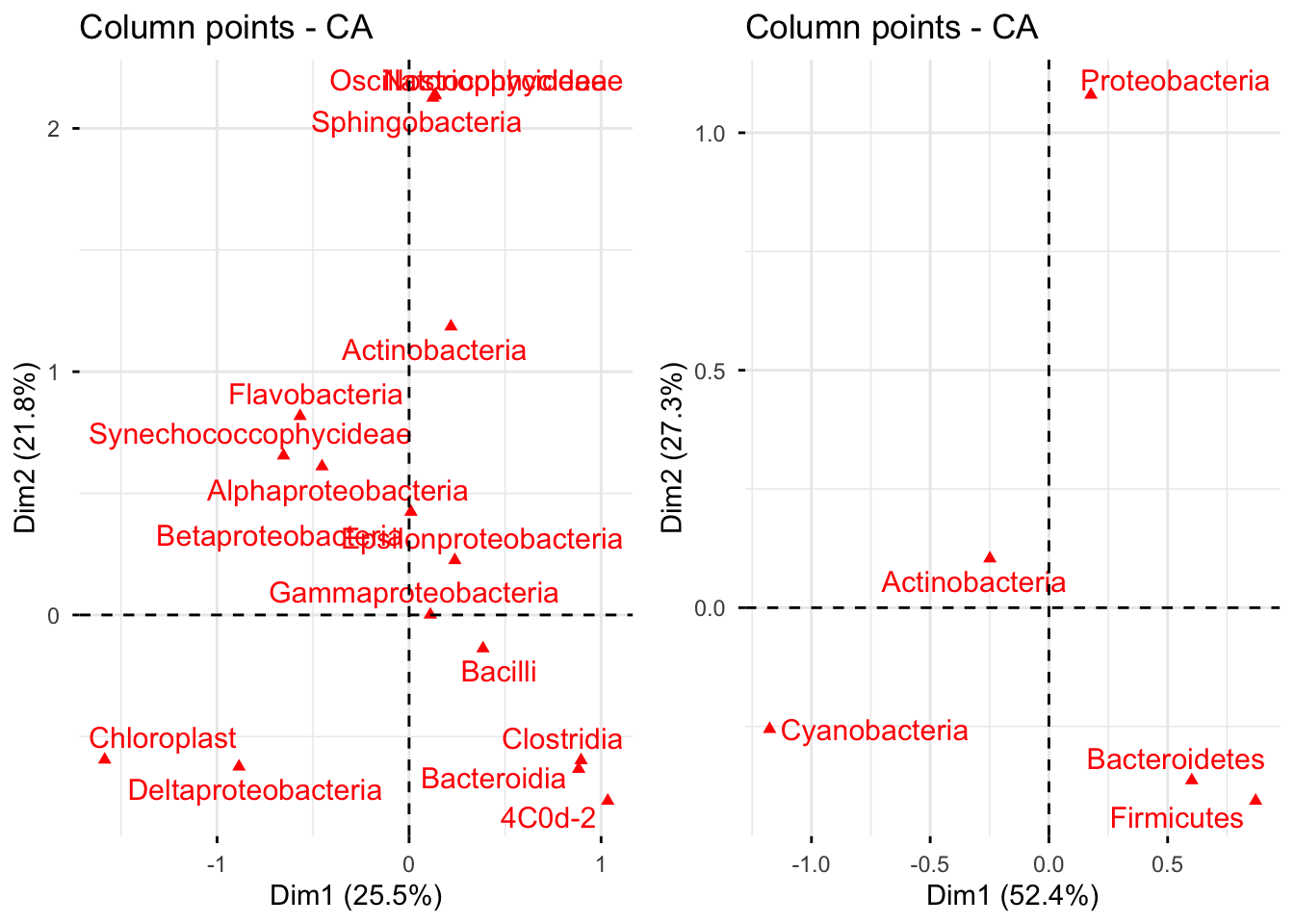
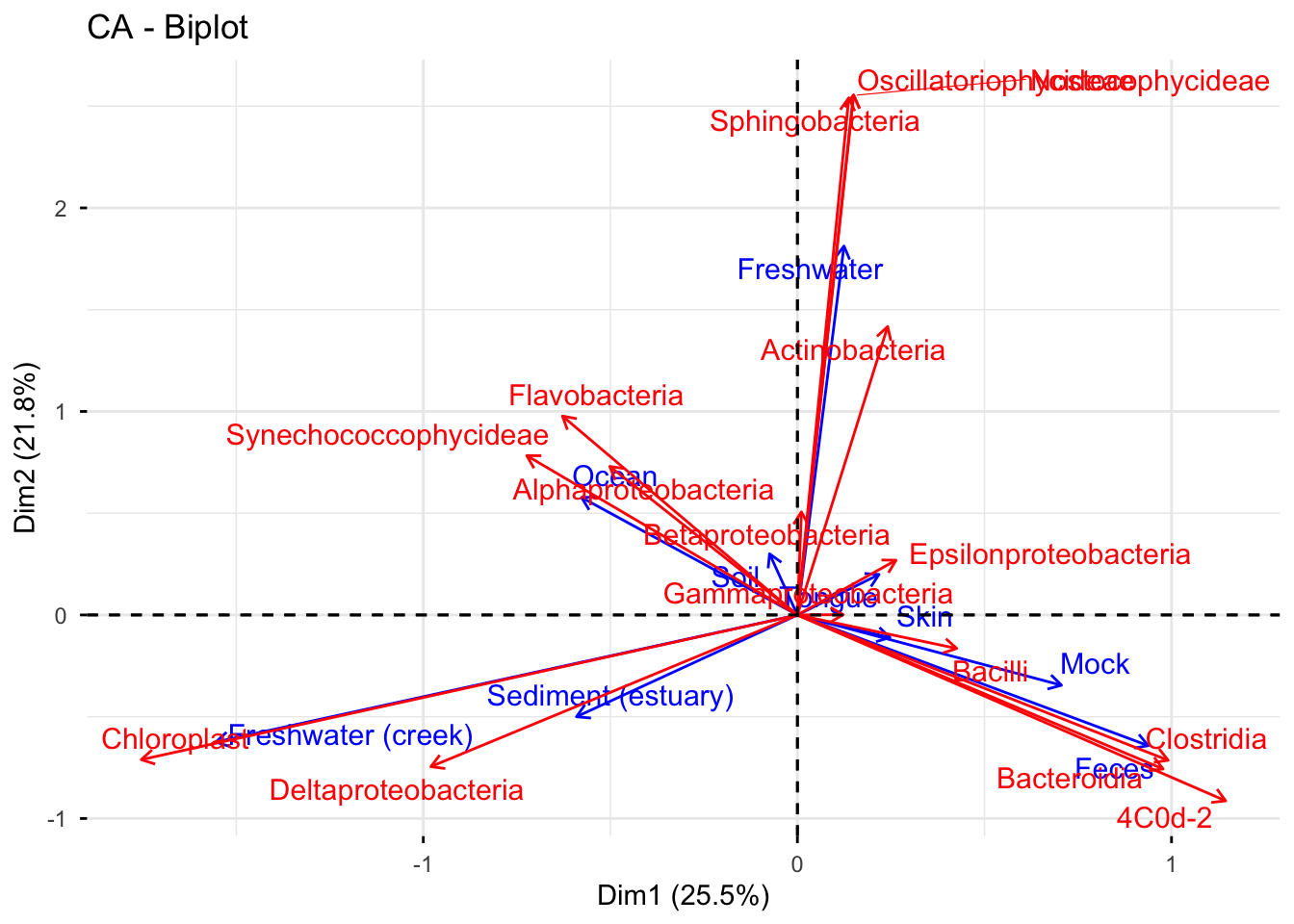
In the first plot, the first dimension is mostly determined by Chloroplast while the second dimension is determined by Oscillatoriophycideae, Nostocophycideae and Sphingobacteria.
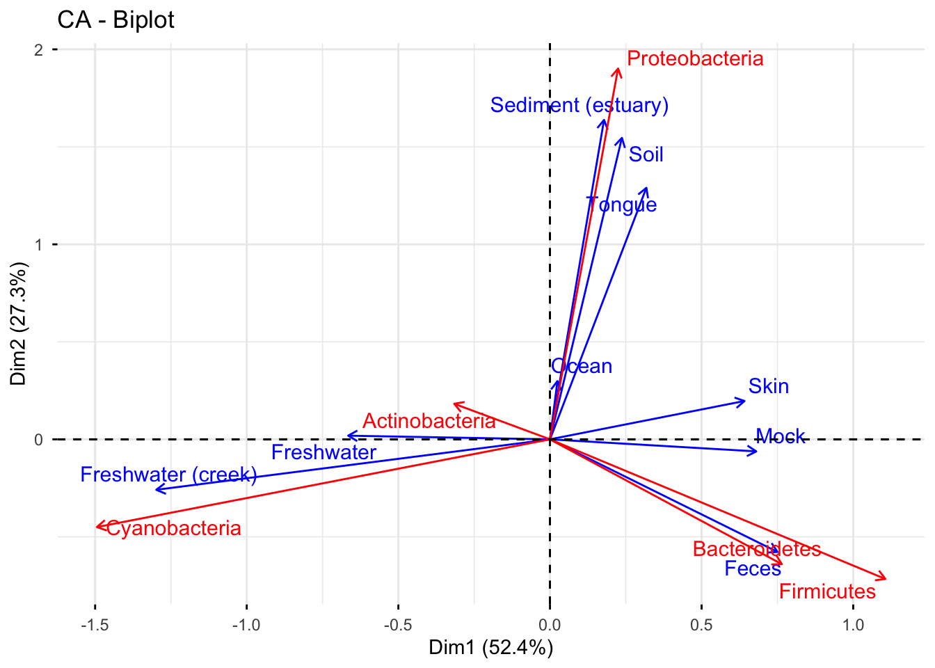
The second graph shows that Cyanobacteria best describes the first dimension and Proteobacteria is the best indicator of the second dimension.
4.3 Biplot Interpretation for Sample Type and Class
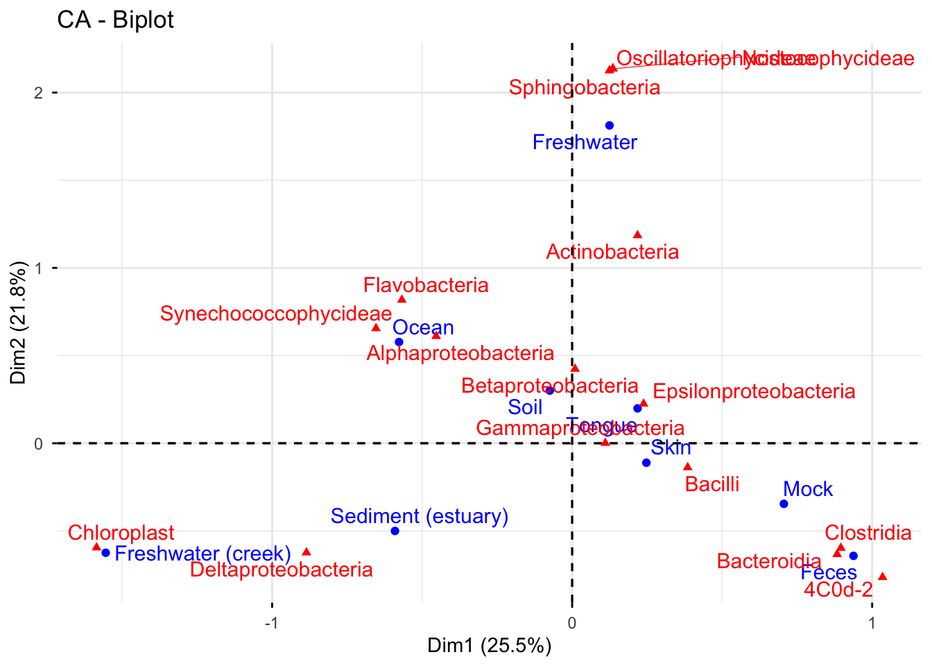
The graph illustrates the distribution of different bacterial classes in various aquatic and terrestrial environments. Oscillatoriophycideae, Nostocophycideae, and Sphingobacteria exhibit a preference for freshwater habitats, while Chloroplast is more commonly found in creek water. Alphaproteobacteria, Flavobacteria, and Synechoccocophycideae display the ability to survive in high-salinity ocean water.
Although Alphaproteobacteria, Betaproteobacteria, and Deltaproteobacteria are all members of the Proteobacteria phylum, Alphaproteobacteria and Betaproteobacteria are primarily found in soil, while Deltaproteobacteria is more commonly found in estuaries.
Epsilonproteobacteria are present in tongue samples, while Clostridia, Bacteroidia, and 4C0d-2 are common bacteria in feces. Bacilli and Clostridia are predominant in the mock, and Gammaproteobacteria and Bacilli tend to colonize human skin
4.4 Biplot Interpretation for Sample Type and Phylum
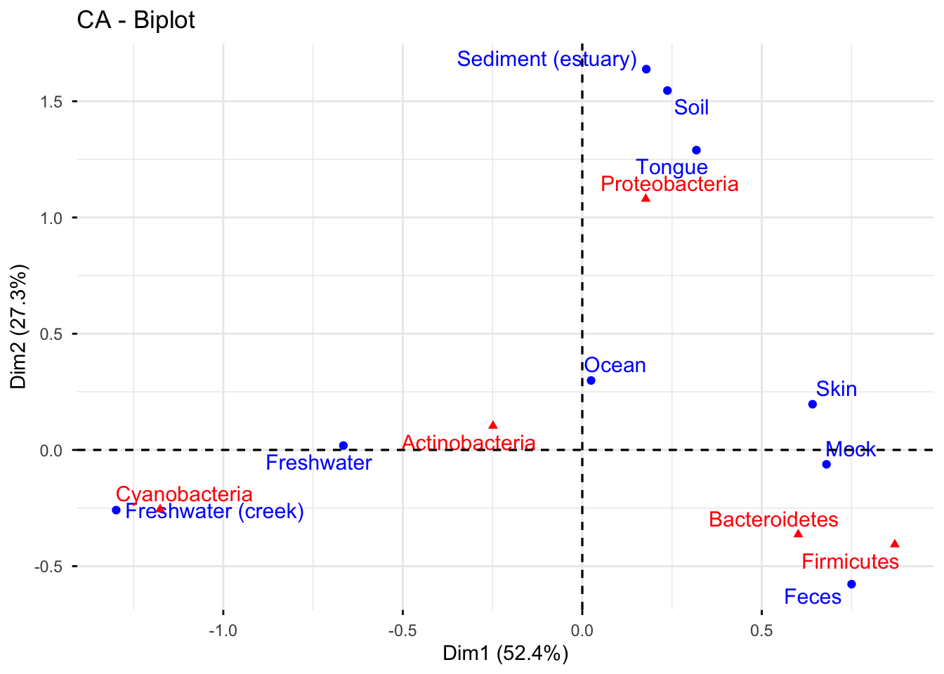
Based on the graph, it can be observed that Proteobacteria is widely distributed in various environments, including human tongue, soil, and estuarine sediment. On the other hand, Cyanobacteria is more commonly found in freshwater creeks. Bacteroides and Firmicutes tend to colonize the human intestinal tract and skin, respectively. Actinobacteria can survive in both freshwater and freshwater(creek) environments.
4.5 Asymmetric Biplot Interpretation for Sample Type and Class
As the asymmetric with row principal coordinates approximate chi square distance of rows, tongue and skin, mock and feces, more or less have similar pattern of bacteria class distributions. In addition, some non-human samples, such as ocean, soil and estuary sediment share some common profiles of bacteria classes.
4.6 Asymmetric Biplot Interpretation for Sample Type and Phylum
Regarding the phyla distribution, there is an apparent separation of samples. These samples then can be divided into three groups: Sediment(estuary), soil, tongue; skin, mock, feces; freshwater and freshwater(creek).
4.7 Interpretation of the Contributions of rows to the dimensions
The graph below show the row contributions of each sample type to dimensions 1 and 2, the sample types that contribute most to a given dimension are the most important in explaining the variability in the data. The red dashed line, indicates the expected average value, If the contributions by all sample types were uniform.
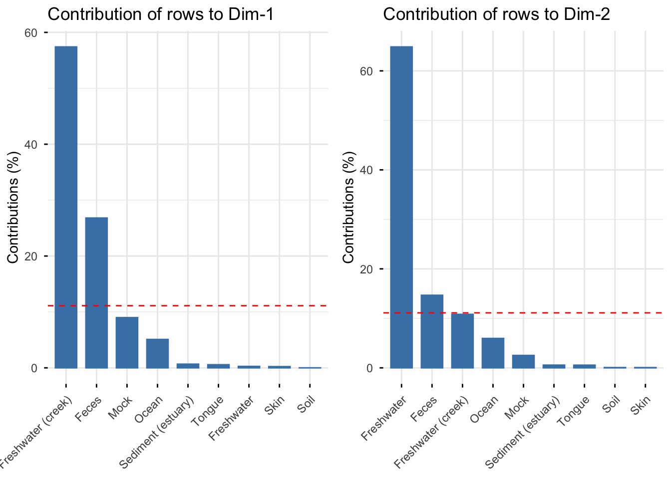
We can see above that dimension 1 is best explained by Freshwater(creek) and Feces while dimension 2 is best explained by Freshwater, Feces and Freshwater(creek), this was also indicated in the original biplot.
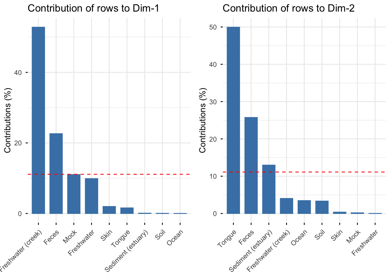
For the dataset showing Sample Type by Phylum, we can see that Freshwater(creek), Feces and Mock best represent dimension 1 and are important in explaining it, while for dimension 2 we see that Tongue, Feces, Sediment (estuary) best explain this dimension.
5. Conclusion
Our results show that there is a significant relationship between row and column categories, with the first two dimensions explaining a substantial amount of the total variation in both matrices.
We found that certain bacterial classes have a preference for specific habitats, such as Oscillatoriophycideae, Nostocophycideae, and Sphingobacteria in freshwater habitats, and Alphaproteobacteria, Flavobacteria, and Synechoccocophycideae in high-salinity ocean water. Clostridia, Bacteroidia, and 4C0d-2 are common in human origin samples. Phyla Bacteriodia and Firmicutes tend to have similar distribution.
Human origin samples i.e., Mock and Feces have same pattern bacteria distribution and while tongue and soil surprisingly share similarities in their bacterial compositions.
Overall, our findings provide valuable insights into the distribution and preference of microbial species in different environments and enhance our understanding of the complex interactions between microbial species and their environments, which has important implications for various fields, including ecology, microbiology, and public health.
References
Caporaso, J. G., et al. (2011). Global patterns of 16S rRNA diversity at a depth of millions of sequences per sample. PNAS, 108, 4516-4522. PMCID: PMC3063599
Greenacre, M. J. (2010). Correspondence analysis. Wiley Interdisciplinary Reviews: Computational Statistics, 2(5), 613-619.
A Practical Guide to the Use of Correspondence Analysis in Marketing Research (M. Bendixen 2003).
Exploratory Multivariate Analysis by Example - Using R (Husson F. et al.)