How to determine the right number of subjects for a two-group experiment using a practical example.
Author
Tom Nangosyah
Published
May 4, 2023
Introduction
One of the most important, yet often overlooked steps in designing an experiment is sample size calculation, if you run your study with very few subjects you risk missing a real effect and when you use many and you waste precious resources and raise ethical concerns.
I took a sample size class as part of my masters in statistics and data science at Uhasselt university and in this short tutorial, I walk through a complete sample size calculation for a two-group experiment.
The example comes from a real-world scenario: a research team wants to compare their experimental Treatment B against the standard-of-care Treatment A by measuring a continuous biomarker score in participants. Their default is 4 participants per group, but is that enough?
We will answer that question by working through the five essential components of any sample size calculation.
The Experimental Setup
The experiment follows a standard two-group design:
Participants are assigned to one of two groups at the start of the study
Each participant receives their assigned treatment over the study period
At the end of the study, the biomarker score is measured for each participant
Two groups are compared:
Group
Treatment
Role
Control
Treatment A
Standard of care
Treatment
Treatment B
Experimental treatment
A reduction of 1.5 units or more in biomarker score would be considered scientifically meaningful. Pilot data from 6 participants assigned to Treatment A are available: 4.6, 6.2, 5.9, 5.3, 6.3, 4.4.
The Five Components of Sample Size Calculation
Every sample size calculation requires specifying five things:
Hypotheses and test
Significance level (\(\alpha\))
Effect size (\(\delta\))
Variance (\(\sigma^2\))
Power (\(1 - \beta\))
Let’s work through each one.
1. Hypotheses and Statistical Test
We want to show that Treatment B reduces the biomarker score compared to Treatment A. Since a lower score is better, we expect \(\mu_{A} > \mu_{B}\) if the new treatment works. This gives us a directional (one-sided) hypothesis:
\[
H_0: \mu_{A} \leq \mu_{B}
\]
\[
H_1: \mu_{A} > \mu_{B}
\]
where \(\mu\) denotes the mean biomarker score in each group.
Why one-sided?
We have a clear scientific expectation about the direction of the effect. We are only interested in detecting whether Treatment B is better than Treatment A, not merely different.
Why a t-test?
Since the population variance is unknown and must be estimated from the data, the appropriate test is a two-sample t-test (not a Z-test). The problem statement confirms that biomarker scores follow a normal distribution, so the t-test assumptions are satisfied.
A Common Mistake: Getting the Direction Wrong
The null hypothesis must contain what you want to disprove. Writing \(H_0: \mu_{A} \geq \mu_{B}\) would flip the meaning since you’d be trying to show that Treatment A is better, which is the opposite of the research question! Always remember: what you want to prove goes in the alternative hypothesis.
2. Significance Level (\(\alpha = 0.05\))
We set \(\alpha = 0.05\), the conventional threshold for controlling the Type I error rate (the probability of concluding Treatment B is better when it actually isn’t). This is the standard choice in research.
3. Effect Size (\(\delta = 1.5\))
The researchers specified that a reduction of 1.5 units in biomarker score would be scientifically relevant. This is our minimum meaningful difference and serves directly as the effect size:
\[
\delta = \mu_{A} - \mu_{B} = 1.5
\]
This value comes from domain expertise and normally it represents the smallest improvement worth detecting.
4. Variance (Standard Deviation)
This is where the pilot data become essential. Let’s compute the standard deviation from the 6 available Treatment A measurements:
The observed SD is approximately 0.82. However, this estimate comes from only 6 participants, so it carries considerable uncertainty. A better approach is to inflate the SD slightly to guard against underestimation. We round up to:
\[
\sigma = 1.0
\]
Why Inflate the Variance?
The pilot study is small (\(n = 6\)), so its variance estimate may be imprecise. A small inflation protects against underestimating the true variability, which would lead to an underpowered study. However, be sure to not over-inflate since the pilot data could also overestimate the true variance, and excessive inflation wastes resources by requiring more participants than necessary.
5. Statistical Power (\(1 - \beta = 0.80\))
We target 80% power, meaning there is an 80% probability of detecting the effect (rejecting \(H_0\)) if the true difference is at least 1.5 units. This is a standard and reasonable choice for discovery-phase experiments.
Computing the Sample Size
With all five components defined, we can compute the required sample size using R’s power.t.test() function. We leave n unspecified so R solves for it:
Code
result <-power.t.test(n =NULL,delta =1.5,sd =1.0,sig.level =0.05,power =0.80,type ="two.sample",alternative ="one.sided",strict =TRUE)result
     Two-sample t test power calculation

              n = 6.298691
          delta = 1.5
             sd = 1
      sig.level = 0.05
          power = 0.8
    alternative = one.sided

NOTE: n is number in *each* group
Code
cat("Required sample size per group:", ceiling(result$n), "\n")
The calculation yields approximately 6.3 per group, which we round up to 7 per group, giving a total of 14 participants.
Is \(n = 4\) Per Group Enough?
The research team’s default is 4 participants per group. Let’s check what power that provides:
Code
check_default <-power.t.test(n =4,delta =1.5,sd =1.0,sig.level =0.05,power =NULL,type ="two.sample",alternative ="one.sided",strict =TRUE)cat("Power with n=4 per group:", round(check_default$power *100, 1), "%\n")
Power with n=4 per group: 59.1 %
With only 4 participants per group, the power is roughly 59% , this would mean there is about a 41% chance of missing a real effect even if Treatment B truly reduces the biomarker score by 1.5 units. This is unacceptably low. The team should increase to at least 7 per group.
Power Curve: Visualizing the Trade-Off
Let’s visualize how power changes with sample size to give the team a fuller picture:
Code
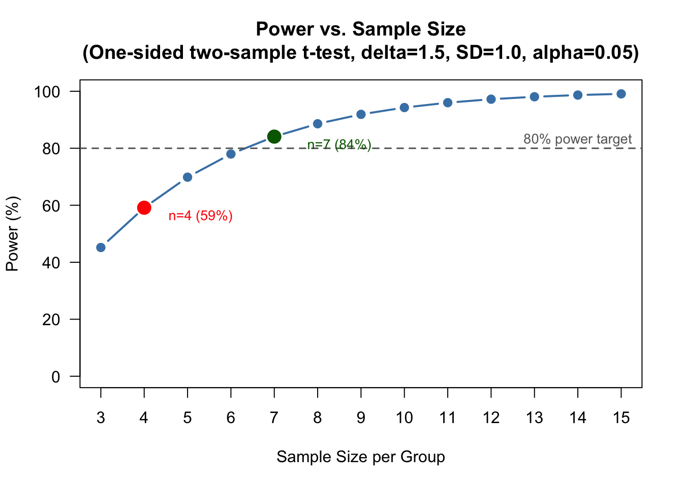
n_range <-3:15power_values <-sapply(n_range, function(n) {power.t.test(n = n, delta =1.5, sd =1.0, sig.level =0.05,type ="two.sample", alternative ="one.sided", strict =TRUE )$power})plot(n_range, power_values *100,type ="b", pch =19, col ="steelblue", lwd =2,xlab ="Sample Size per Group",ylab ="Power (%)",main ="Power vs. Sample Size\n(One-sided two-sample t-test, delta=1.5, SD=1.0, alpha=0.05)",ylim =c(0, 100),las =1, xaxt ="n")axis(1, at = n_range)abline(h =80, lty =2, col ="gray40", lwd =1.5)text(14, 83, "80% power target", col ="gray40", cex =0.85)points(4, power_values[n_range ==4] *100, col ="red", pch =19, cex =1.8)text(5.3, power_values[n_range ==4] *100-3, "n=4 (59%)", col ="red", cex =0.85)points(7, power_values[n_range ==7] *100, col ="darkgreen", pch =19, cex =1.8)text(8.5, power_values[n_range ==7] *100-3, "n=7 (84%)", col ="darkgreen", cex =0.85)
Statistical power as a function of sample size per group. The dashed line marks the 80% power target; the red dot indicates the team’s default of n=4.
The curve shows diminishing returns: going from 4 to 7 participants yields a large power gain (approx. 25%), but each additional participant beyond 7 contributes less.
Sensitivity Analysis: What If Our SD Estimate Is Off?
Since the variance estimate comes from a small pilot, it’s worth checking how the sample size changes under different assumptions:
Code
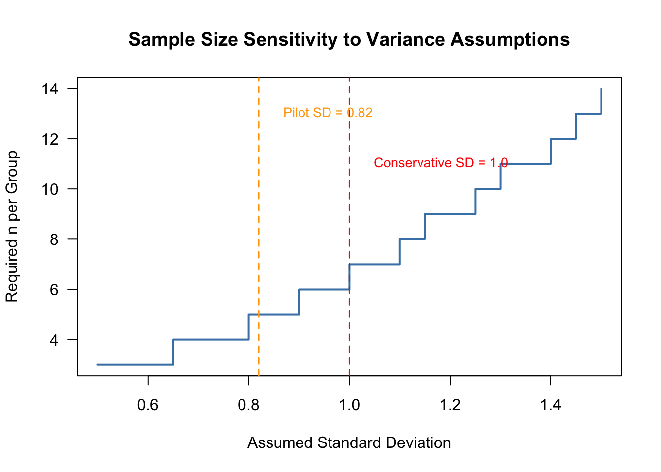
sd_range <-seq(0.5, 1.5, by =0.05)n_required <-sapply(sd_range, function(s) {ceiling(power.t.test(n =NULL, delta =1.5, sd = s, sig.level =0.05, power =0.80,type ="two.sample", alternative ="one.sided", strict =TRUE )$n)})plot(sd_range, n_required,type ="s", col ="steelblue", lwd =2,xlab ="Assumed Standard Deviation",ylab ="Required n per Group",main ="Sample Size Sensitivity to Variance Assumptions",las =1)abline(v =0.82, lty =2, col ="orange", lwd =1.5)text(0.85, max(n_required) -1, "Pilot SD = 0.82", col ="orange", pos =4, cex =0.85)abline(v =1.0, lty =2, col ="red", lwd =1.5)text(1.03, max(n_required) -3, "Conservative SD = 1.0", col ="red", pos =4, cex =0.85)
Required sample size per group across a range of assumed standard deviations. Vertical lines mark the observed pilot SD (0.82) and the conservative estimate (1.0).
This highlights why a conservative SD estimate matters, we see that if the true SD is even slightly larger than 0.82, the required sample size increases quickly.
Summary of sample size calculation parameters and result.
Component
Specification
Null hypothesis
mu_A <= mu_B
Alternative hypothesis
mu_A > mu_B
Statistical test
One-sided two-sample t-test
Significance level (alpha)
0.05
Effect size (delta)
1.5 units (biomarker score)
Standard deviation (sigma)
1.0 (inflated from pilot SD = 0.82)
Power (1 - beta)
80%
Result: n per group
7
Result: Total N
14
Key Takeaways
Always perform a sample size calculation before running an experiment. The team’s default of 4 participants per group would only provide about 59% power which is barely better than a coin flip at detecting a real effect.
The five ingredients are non-negotiable: hypotheses/test, significance level, effect size, variance, and power. Each must be justified.
Be conservative with variance estimates from small pilots, but don’t over-inflate. Rounding from SD = 0.82 to SD = 1.0 is a reasonable decision.
A one-sided test is appropriate when the research question is directional. Here, we only care about Treatment B being better than Treatment A.
The answer: use at least 7 participants per group (14 total) to achieve 80% power for detecting a 1.5-unit reduction in biomarker score.