Formula One Performance DNA (Japan Update)

After the first two races I published a performance tier analysis that used sector times, top speed, qualifying pace, and race pace to cluster the eleven 2026 teams into four competitive groups. The analysis received a really sharp observation from a reader that I had not paid close attention to given the change in regulations in the new season:

“The current Formula One Regulations are predominantly dependent on Energy deployment of the battery. The 50/50 split between Internal Combustion Engine and Electric Power creates further complications in assessing peak horsepower of the different teams. The speed through the mid and high speed corners may not provide the best data as well as teams and cars are not moving at full speed as they manage battery deployment. There is further complexity with the cars having to super-clip to harvest energy at the end of each straight and losing straight line speed despite the driver being at full throttle.”

I will start by defining Super Clipping, in F1 this yearthis refers to a technical phenomenon where the cars harvest energy for their high-output hybrid batteries while the driver is still at full throttle, rather than traditional energy recovery under braking.

In the original raw SpeedST (speed-trap readings on the main straight) was used as a proxy for straight-line pace. When a car is harvesting energy it will show a lower SpeedST reading even at full driver throttle. That makes aggressive harvesters look slower on the straight than they actually are, which farther would bias the top-speed and power-sector dimensions of the DNA profile that we developed earlier.

This updated analysis adds the Japanese Grand Prix (Suzuka, Round 3) and introduces two methodological corrections to address the hybrid complication:

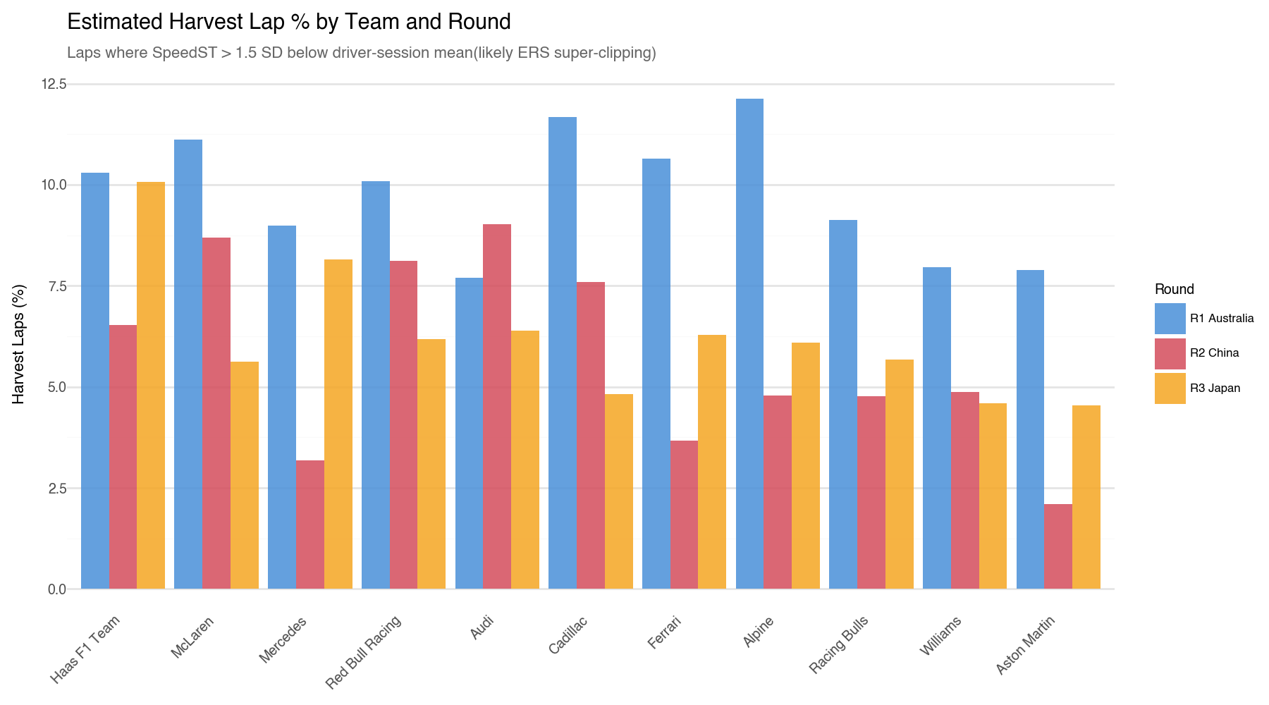
1. Harvest-lap flagging, here laps where SpeedST is more than 1.5 standard deviations below the driver’s own session mean are flagged as likely super-clip laps. Their speed readings are replaced with an imputed value (the driver’s 85th percentile speed in that session) before entering the top-speed dimension.
2. Power-sector down-weighting, in non-qualifying sessions, the power-sector time readings will receive a 20% reduction in the aggregation step, because Energy Recovery System harvesting has the most distorting effect in these sectors. Qualifying sessions are exempt as teams deploy maximum Energy Recovery in qualifying, so those readings represent true car pace.

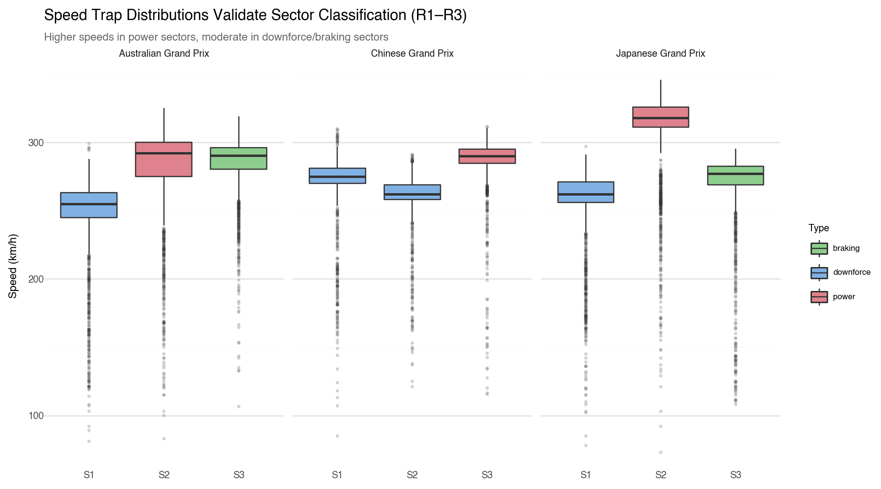
Suzuka itself adds useful signal, Sector 1 normally called “the Esses” requires pure mechanical grip and minimal ERS involvement.

Caveat - three races is still a small sample

Melbourne, Shanghai and Suzuka test overlapping but different skills. The corrections below are just approximations, the profile will continue to stabilise as more circuits accumulate.

Data Collection

We extend the existing pipeline to include all standard sessions for the Japanese Grand Prix weekend.

YEAR = 2026

# Chinese GP is a Sprint weekend; Australia and Japan are standard.
RACES = {
    "Australian Grand Prix": ["FP1", "FP2", "FP3", "Q", "Race"],
    "Chinese Grand Prix":    ["FP1", "SQ", "S", "Q", "Race"],
    "Japanese Grand Prix":   ["FP1", "FP2", "FP3", "Q", "Race"],
}

KEEP_COLS = [
    "Driver", "DriverNumber", "Team", "LapNumber", "LapTime",
    "Sector1Time", "Sector2Time", "Sector3Time",
    "SpeedI1", "SpeedI2", "SpeedFL", "SpeedST",
    "Compound", "TyreLife", "FreshTyre",
    "IsPersonalBest", "Deleted", "IsAccurate",
]

all_laps = []
for race_name, session_types in RACES.items():
    for stype in session_types:
        try:
            session = fastf1.get_session(YEAR, race_name, stype)
            session.load()
        except Exception as e:
            print(f"  [{race_name} | {stype}] Skipped: {e}")
            continue
        lap_data = session.laps
        if lap_data is None or len(lap_data) == 0:
            continue
        available = [c for c in KEEP_COLS if c in lap_data.columns]
        df = lap_data[available].copy()
        df["Year"]        = YEAR
        df["RaceName"]    = race_name
        df["Round"]       = session.event["RoundNumber"]
        df["CircuitName"] = session.event["Location"]
        df["SessionType"] = stype
        all_laps.append(df)

combined = pd.concat(all_laps, ignore_index=True)

Controlling for the Battery Effect

This is the core problem. Under the 2026 rules, roughly half the car’s power comes from the battery. When the battery is full, the car switches to charging mode and even with the driver flat on the throttle, the car goes slower than it normally would. That makes some laps look slow on the speed trap even though the car itself isn’t actually slow.

We deal with this in two simple steps:

1. We find the affected laps, if a driver’s speed-trap reading is much lower than their own typical speed in that same session, we flag it as a likely harvest lap.
2. We replace the bad reading, instead of throwing the lap away, we swap in that driver’s best typical speed from the session, so it no longer pulls the team’s score down unfairly.

Finding the harvest laps

def flag_harvest_laps(laps_df, z_thresh=1.5):
    """
    Flag laps where SpeedST is anomalously low — indicating ERS harvest
    (super-clipping) rather than a genuine slow straight-line speed.
    """
    df = laps_df.copy()
    if "SpeedST" not in df.columns:
        df["HarvestLap"]    = False
        df["SpeedST_ZScore"] = np.nan
        return df

    grp = ["Round", "Driver", "SessionType"]
    df["SpeedST_Mean"]   = df.groupby(grp)["SpeedST"].transform("mean")
    df["SpeedST_Std"]    = df.groupby(grp)["SpeedST"].transform("std")
    df["SpeedST_ZScore"] = np.where(
        df["SpeedST_Std"] > 0,
        (df["SpeedST"] - df["SpeedST_Mean"]) / df["SpeedST_Std"],
        0.0,
    )
    df["HarvestLap"] = df["SpeedST_ZScore"] < -z_thresh
    df = df.drop(columns=["SpeedST_Mean", "SpeedST_Std"])
    return df

laps_flagged = flag_harvest_laps(laps)

This chart reveals interesting variation across teams and circuits. Teams with higher harvest percentages are managing their battery more actively, which tells us about strategy, not pace, but it matters because without correction those laps drag down their power-sector and top-speed scores unfairly.

Replacing the bad readings

For any lap flagged as a harvest lap, we swap in the driver’s typical best speed from that session, essentially, what this car normally does on the straight when it is not charging.

def hybrid_corrected_top_speed(laps_df, z_thresh=1.5):
    """
    Compute team top speed with harvest-lap correction.
    Harvest laps have SpeedST imputed as the driver's p85 session speed.
    """
    df = flag_harvest_laps(laps_df, z_thresh)
    if "SpeedST" not in df.columns:
        return pd.Series(dtype=float, name="top_speed_corrected")

    # p85 reference speed per driver-session
    p85 = (
        df[~df["HarvestLap"]]
        .groupby(["Round", "Driver", "SessionType"])["SpeedST"]
        .quantile(0.85)
        .rename("SpeedST_p85")
        .reset_index()
    )
    df = df.merge(p85, on=["Round", "Driver", "SessionType"], how="left")

    df["SpeedST_corrected"] = np.where(
        df["HarvestLap"] & df["SpeedST_p85"].notna(),
        df["SpeedST_p85"],
        df["SpeedST"],
    )

    team_speed    = df.groupby("Team")["SpeedST_corrected"].median()
    median_speed  = team_speed.median()
    top_speed_cor = (team_speed / median_speed) * 100 - 100
    top_speed_cor.name = "top_speed_corrected"
    return top_speed_cor

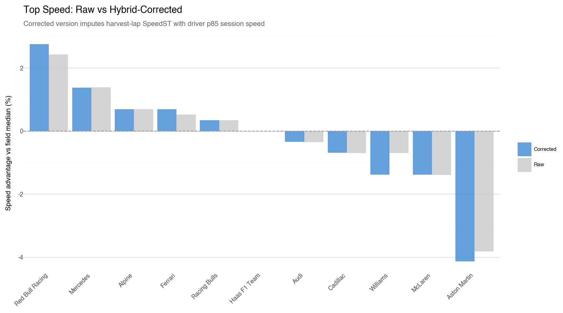
Teams that harvest most aggressively see the largest upward correction, their true straight-line pace is better than the raw data suggested. Teams that rarely harvest are largely unaffected.

Classifying Sectors (We add Suzuka)

We now classify sectors across all three circuits.

SECTOR_CLASSIFICATION = {
    "Melbourne": {
        1: "downforce",   # turns 1-4: medium-speed technical corners
        2: "power",       # high-speed sweepers + back straight
        3: "braking",     # heavy braking into chicanes
    },
    "Shanghai": {
        1: "downforce",   # tight/twisty turns 1-4
        2: "downforce",   # medium-high speed section (turns 5-10)
        3: "power",       # 1.2 km back straight
    },
    "Suzuka": {
        1: "downforce",   # Esses + Degner — pure aero/mechanical grip
        2: "power",       # back straight + Spoon — ERS deployment zone
        3: "braking",     # Hairpin + Casio chicane — heavy braking complex
    },
}

def get_sector_type(circuit_name, sector_num):
    for key, sectors in SECTOR_CLASSIFICATION.items():
        if key.lower() in circuit_name.lower():
            return sectors.get(sector_num, "mixed")
    return "mixed"

Normalising Sector Performance (with Hybrid Weighting)

The normalisation approach is the same as before, we express each sector time as a percentage of the field median, but we now apply an additional discount to power-sector readings in non-qualifying sessions.

SESSION_WEIGHTS = {
    "Q": 3.0, "Race": 2.0, "S": 2.0,
    "SQ": 1.5,
    "FP1": 1.0, "FP2": 1.0, "FP3": 1.0,
}

def hybrid_adjusted_weight(session_type, sector_type):
    """
    Power-sector laps in non-qualifying sessions are down-weighted by 20 %
    because ERS harvest distorts straight-line speed readings in exactly
    those sectors.  Qualifying is exempt: teams run maximum ERS deployment
    so the readings represent true car pace.
    """
    base = SESSION_WEIGHTS.get(session_type, 1.0)
    if session_type != "Q" and sector_type == "power":
        return base * 0.8
    return base

def normalize_sector_times(df, group_cols, sector_col):
    median = df.groupby(group_cols)[sector_col].transform("median")
    return (df[sector_col] / median) * 100

(
    ggplot(
        sectors.dropna(subset=["MeanSpeed"]),
        aes(x="SectorLabel", y="MeanSpeed", fill="SectorType"),
    )
    + geom_boxplot(alpha=0.7, outlier_alpha=0.15, outlier_size=0.5)
    + facet_wrap("~RaceName")
    + scale_fill_manual(values=sector_palette)
    + labs(
        title="Speed Trap Distributions Validate Sector Classification (R1–R3)",
        subtitle="Higher speeds in power sectors, moderate in downforce/braking sectors",
        x="",
        y="Speed (km/h)",
        fill="Type",
    )
    + car_dna_theme
)

Building the Performance Profile

Qualifying Pace

q_laps = laps[laps["SessionType"] == "Q"].dropna(subset=["LapTimeSec"])
pb = (
    q_laps
    .groupby(["Round", "RaceName", "Driver", "Team"])["LapTimeSec"]
    .min()
    .reset_index()
    .rename(columns={"LapTimeSec": "QualiBestSec"})
)
for rnd in pb["Round"].unique():
    mask = pb["Round"] == rnd
    field_median = pb.loc[mask, "QualiBestSec"].median()
    pb.loc[mask, "NormQuali"] = (pb.loc[mask, "QualiBestSec"] / field_median) * 100

team_quali = (
    pb.groupby(["Round", "Team"])["NormQuali"].min()
    .groupby("Team").mean()
)
quali_mean = team_quali.mean()
qualifying_pace = quali_mean - team_quali
qualifying_pace.name = "qualifying_pace"

Race Pace

race = laps[laps["SessionType"] == "Race"].dropna(subset=["LapTimeSec"]).copy()
if "IsAccurate" in race.columns:
    race = race[race["IsAccurate"] == True]
if "TyreLife" in race.columns:
    race = race[race["TyreLife"] > 1]
driver_med = race.groupby(["Round", "Driver"])["LapTimeSec"].transform("median")
race = race[race["LapTimeSec"] <= driver_med * 1.07]

for rnd in race["Round"].unique():
    mask = race["Round"] == rnd
    field_median = race.loc[mask, "LapTimeSec"].median()
    race.loc[mask, "NormRace"] = (race.loc[mask, "LapTimeSec"] / field_median) * 100

team_race = race.groupby("Team")["NormRace"].median()
race_mean = team_race.mean()
race_pace = race_mean - team_race
race_pace.name = "race_pace"

Assembling the Profile

from great_tables import GT, style, loc

(
    GT(dna.round(2))
    .tab_header(
        title="Performance Profile (Rounds 1-3)",
        subtitle="Teams ranked by overall score. Top speed dimension corrected for ERS harvest laps.",
    )
    .cols_label(
        braking_sector="Braking",
        downforce_sector="Downforce",
        power_sector="Power",
        top_speed="Top Speed",
        qualifying_pace="Qualifying",
        race_pace="Race Pace",
        overall_score="Overall",
    )
    .tab_spanner(label="Sector Performance", columns=["braking_sector", "downforce_sector", "power_sector"])
    .tab_spanner(label="Performance Metrics", columns=["top_speed", "qualifying_pace", "race_pace"])
    .tab_style(
        style=[style.fill(color="#d4edda"), style.text(weight="bold")],
        locations=loc.body(
            rows=lambda df: df["overall_score"] >= df["overall_score"].nlargest(3).min()
        ),
    )
    .tab_style(
        style=style.fill(color="#f8d7da"),
        locations=loc.body(
            rows=lambda df: df["overall_score"] <= df["overall_score"].nsmallest(3).max()
        ),
    )
    .tab_source_note(
        "Top speed corrected for ERS harvest laps (super-clip imputation). "
        "Power-sector weights ×0.8 in non-qualifying sessions."
    )
)

Performance Profile (Rounds 1-3)
Teams ranked by overall score. Top speed dimension corrected for ERS harvest laps.
Team	Sector Performance			Performance Metrics			Overall
	Braking	Downforce	Power	Top Speed	Qualifying	Race Pace
Mercedes	3.36	3.13	3.05	1.38	1.79	2.07	2.46
Red Bull Racing	2.55	0.97	1.52	2.76	0.68	0.38	1.48
Ferrari	0.62	1.01	-0.07	0.69	1.13	1.57	0.82
McLaren	0.07	0.75	-0.25	-1.38	1.12	1.65	0.33
Alpine	-0.88	-0.42	-0.1	0.69	0.34	-0.15	-0.09
Haas F1 Team	-0.23	-0.94	0.19	0.0	0.07	-0.02	-0.16
Racing Bulls	-1.29	0.04	-0.58	0.34	0.08	-0.01	-0.23
Audi	-0.29	-1.11	-1.12	-0.34	0.17	-0.06	-0.46
Williams	0.1	-0.58	-0.84	-1.38	-0.82	-0.58	-0.68
Cadillac	-2.02	-1.22	-0.12	-0.69	-2.38	-1.94	-1.4
Aston Martin	-1.99	-1.62	-1.68	-4.14	-2.2	-2.91	-2.42
Top speed corrected for ERS harvest laps (super-clip imputation). Power-sector weights ×0.8 in non-qualifying sessions.

The Performance Profile Map

from sklearn.preprocessing import StandardScaler
from plotnine import ggplot, aes, geom_tile, geom_text, scale_fill_gradient2, labs, theme, element_text

feature_cols = [
    "braking_sector", "downforce_sector", "power_sector",
    "top_speed", "qualifying_pace", "race_pace",
]
scaler = StandardScaler()
dna_scaled = dna.copy()
dna_scaled[feature_cols] = scaler.fit_transform(dna[feature_cols].fillna(0))

dim_labels = {
    "braking_sector":   "Braking",
    "downforce_sector": "Downforce",
    "power_sector":     "Power",
    "top_speed":        "Top Speed",
    "qualifying_pace":  "Quali Pace",
    "race_pace":        "Race Pace",
}

dna_heat = dna_scaled.melt(
    id_vars="Team",
    value_vars=feature_cols,
    var_name="Dimension",
    value_name="ZScore",
)
dna_heat["DimLabel"] = dna_heat["Dimension"].map(dim_labels)

team_order = (
    dna_heat.groupby("Team")["ZScore"]
    .mean()
    .sort_values(ascending=False)
    .index.tolist()
)
dna_heat["Team"] = pd.Categorical(dna_heat["Team"], categories=team_order, ordered=True)

(
    ggplot(dna_heat, aes(x="DimLabel", y="Team", fill="ZScore"))
    + geom_tile(color="white", size=0.8)
    + geom_text(aes(label="round(ZScore, 1)"), size=6, color="#333333")
    + scale_fill_gradient2(low="#D44D5C", mid="#F5F5F5", high="#5CB85C", midpoint=0)
    + labs(
        title="Performance Profile Heatmap (Rounds 1–3)",
        subtitle="Green = strength, Red = weakness. Top Speed = corrected for ERS harvest.",
        x="",
        y="",
        fill="Z-Score",
    )
    + theme(
        figure_size=(9, 6),
        axis_text_x=element_text(rotation=30, ha="right", size=7),
    )
    + car_dna_theme
)

Clustering

fig, ax = plt.subplots(figsize=(10, 5))
dendrogram(
    linkage_matrix,
    labels=teams,
    leaf_rotation=35,
    leaf_font_size=8,
    ax=ax,
    color_threshold=5,
)
ax.set_title(
    "Team Performance DNA Dendrogram - Rounds 1–3 (Ward Linkage)",
    fontsize=10, fontweight="bold",
)
ax.set_ylabel("Distance", fontsize=8)
ax.axhline(y=5, color="#D44D5C", linestyle="--", alpha=0.5, label="Cluster cut")
ax.legend(fontsize=7)
ax.tick_params(labelsize=7)
plt.tight_layout()
plt.show()

Race Results

Team	Australia	China	Japan
Mercedes	1st, 2nd	1st, 2nd	1st, 4th
McLaren	5th, DNS	DNS, DNS	2nd, 5th
Ferrari	3rd, 4th	3rd, 4th	3rd, 6th
Alpine	10th	6th	7th, 16th
Red Bull	6th, DNF	8th, DNF	8th, 12th
Racing Bulls	8th	7th	9th, 14th
Haas	7th	5th	10th, Ret
Audi	9th	DNS	11th, 13th
Williams	12th, 15th	DNS	15th, 20th (lapped)
Cadillac	16th, DNF	13th, 15th	17th, 19th (lapped)
Aston Martin	DNF, NC	DNF, DNF	18th (lapped), Ret

What Changed ?

Comparing the R3 analysis to the R2 version:

• Top-speed dimension shifted upward for teams that harvest most aggressively. If a team routinely super-clips through practice and race sessions, their raw SpeedST median was artificially reduced, the correction restores a fairer picture of their actual straight-line capability.
• Power-sector scores are slightly more stable because the 0.8 × discount reduces the influence of harvest-contaminated practice sessions and lets qualifying data carry more of the difference.
• The Suzuka Esses (S1) provides a harvest-free reference point. Relative performance in that sector should be treated as reliable readings in this analysis.

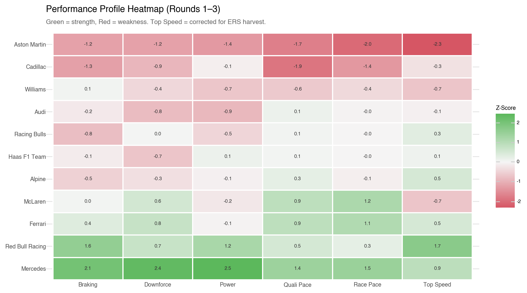
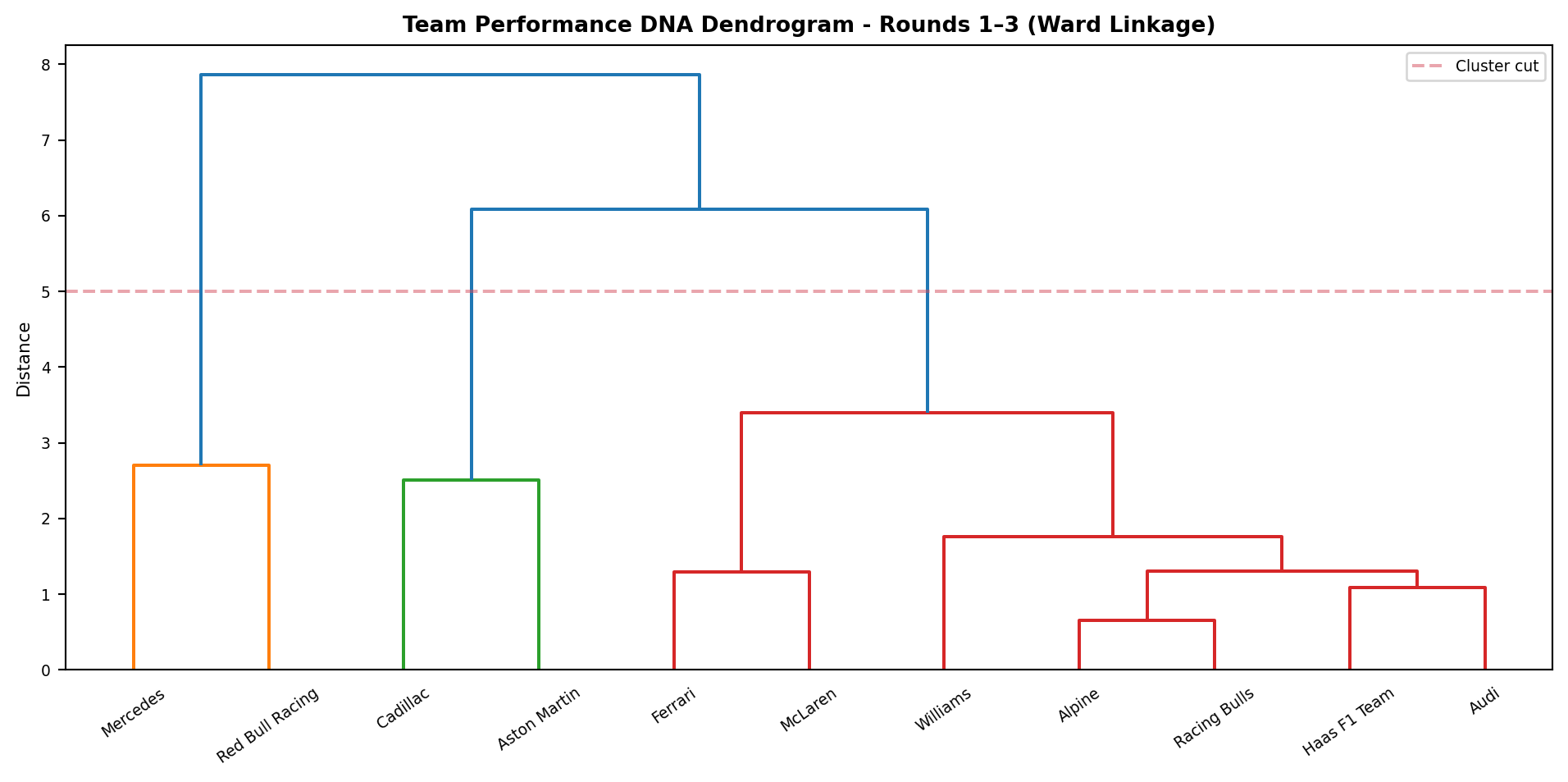
The clustering group assignments are expected to remain broadly similar to the R2 analysis, but the distances within and between groups should be more reliable now that the ERS problem has been partly addressed.

Limitations

Overall, the analysis gives useful insights but isn’t precise. The results are influenced by assumptions, limited data, and track-specific factors, so they should be seen as indicative trends rather than exact measures of car performance. As more varied race data becomes available, the conclusions will become more reliable.

Note on AI Use

AI tools were used to support coding, generate visualisations, and help debug sections of code. All decisions, interpretations, and insights presented here are the result of personal analysis.