A tiny end-to-end ML pipeline for Kiva Loans

This is a small, low stakes example of building a complete machine learning pipeline in Python, from pulling raw data off a public API all the way to a working app that serves live predictions. Nothing here is meant to be taken too seriously. The dataset is small, the model is simple, and several of the modeling choices below were made for convenience.

The point of the exercise is to show the shape of a pipeline: extract, tidy, train, evaluate, deploy, serve, using tools from the Posit ecosystem (pins, vetiver, and Shiny for Python) to hold it together.

flowchart LR
    A["Extract\nkiva_extract.py"] --> B["Tidy\ntransform.py"]
    B --> C["Train\ntrain.py"]
    C --> D["Evaluate\nevaluate.py"]
    C --> E["Deploy\ndeploy.py"]
    E --> F["Serve\napp.py"]

The data: microloans from Uganda

The data comes from Kiva, a nonprofit that connects lenders with small businesses and entrepreneurs, mostly in low income countries. Each listing includes a short, free text description, written by a Kiva field partner on the borrower’s behalf, describing what the loan will actually be used for. Something like “to buy fertilizer to improve her soil for healthy coffee growing.”

I pulled about 2,000 loan listings from Uganda using Kiva’s public API. The task I picked: predict which broad sector a loan belongs to (agriculture, business, or personal use) just from that short description.

Important

This pipeline predicts sector labels. I use this example typically for illustration purposes.

import pandas as pd
import pins
from sklearn.compose import ColumnTransformer
from sklearn.dummy import DummyClassifier
from sklearn.feature_extraction.text import TfidfVectorizer
from sklearn.linear_model import LogisticRegression
from sklearn.metrics import accuracy_score, classification_report, confusion_matrix, f1_score
from sklearn.model_selection import StratifiedKFold, cross_validate, train_test_split
from sklearn.pipeline import Pipeline
from sklearn.preprocessing import StandardScaler
import numpy as np

board = pins.board_folder("pins_board", allow_pickle_read=True)
tidy = board.pin_read("kiva_tidy_loans")
tidy[["sector", "sector_grouped", "use"]].head()

	sector	sector_grouped	use
0	Agriculture	Agriculture	to buy fertilizers to improve soils for health...
1	Agriculture	Agriculture	to buy manure to improve soils to grow healthy...
2	Retail	Business	to add stock to the business.
3	Agriculture	Agriculture	to buy seedlings to diversify her crops and in...
4	Agriculture	Agriculture	to buy seedlings to diversify his crops and in...

Step 1: pulling data from an API

The extraction step (kiva_extract.py in the repo) loops over Kiva’s loans/search endpoint and collects four pages of 500 loans each, filtered to Uganda.

This step is also the most fragile part of the whole pipeline, since it depends entirely on a third party API staying available and unchanged. That is worth keeping in mind for any pipeline that starts with “pulling data from someone else’s website.”

Step 2: tidying the data and picking a target

Kiva’s own sector labels are much finer grained than what we use here, eighteen categories in total, ranging from Agriculture (over 800 loans) down to sectors with a single loan. Modeling eighteen classes with that kind of imbalance is not a great use of anyone’s time, so I made a judgment call to merge the rare sectors together, then group everything into three broader buckets.

tidy["sector_grouped"].value_counts()

sector_grouped
Agriculture    805
Personal       700
Business       495
Name: count, dtype: int64

That grouping (Agriculture on its own, Retail and Services combined into Business, everything else combined into Personal) is not an official Kiva taxonomy. It is a modeling convenience chosen to get a more balanced, more tractable classification problem. If you needed the original fine grained sectors for a real application, you would want to handle the class imbalance properly (more data, resampling, hierarchical classification) rather than merging categories away.

Step 3: why bag of words ?

The business question here is deliberately simple: given a short sentence describing what a loan is for, guess one of three broad categories. That kind of question does not need a sophisticated model to answer reasonably well, so it is worth starting with the simplest thing that could plausibly work before reaching for anything heavier.

Bag of words, means throwing away word order and grammar, and just counting which words show up in each description. “to buy fertilizer for coffee” and “fertilizer to buy for coffee” look identical to a bag of words model, since it only sees a big table of word counts, one row per loan, one column per word. TF-IDF (the variant used here) is a small refinement on plain counts: it downweights words that show up in almost every description (like “to” or “buy”) and upweights words that are distinctive to a smaller set of loans (like “fertilizer” or “merchandise”), since the distinctive words tend to be more useful for telling categories apart.

Logistic regression, then learns a weight for each of those word columns, one set of weights per sector. To classify a new description, it multiplies each word’s count by its learned weight, adds those up, and picks whichever sector gets the highest score. A positive weight on “fertilizer” for Agriculture just means: the more that word count, the more this model leans toward calling it Agriculture. That is also why it is easy to inspect afterwards, as in the table below, the weights themselves tell you exactly which words are driving each prediction.

Why this combination, specifically, for this problem:

• The use field is short and fairly templated. Field partners tend to write structured phrases like “to buy X to do Y,” not free flowing prose, so word order carries little extra information beyond the words themselves.
• The vocabulary is concrete and sector specific. Borrowers do not describe abstract plans, they describe fertilizer, cows, shop stock, and school fees, which is exactly the kind of signal a word-count model can pick up directly.
• The dataset is small (2,000 rows). Bag of words plus logistic regression needs relatively little data to find signal and stays fully interpretable, which makes it a sensible starting point before considering anything like word embeddings or transformer-based language models.
• In many low income country contexts, the infrastructure to run larger NLP models is not always readily available, and would not be worth the operational cost for a problem this small. A linear model over word counts is cheap to train, cheap to serve, and easy to explain to a non technical stakeholder.

To be clear, this is a that was made out of convenience for illustration, not a claim that bag of words is the best possible approach to text classification in general. The point here is to show a complete, working pipeline end to end, not to squeeze out the best possible accuracy.

Here is a look at some of the vocabulary the model actually leans on for each sector:

X = tidy[["use"]]
y = tidy["sector_grouped"]

X_train, X_test, y_train, y_test = train_test_split(
    X, y, test_size=0.2, random_state=2984, stratify=y,
)

text_pipe = Pipeline([
    ("preprocessor", ColumnTransformer([
        ("use_text", TfidfVectorizer(max_features=300, stop_words="english"), "use"),
    ])),
    ("model", LogisticRegression(class_weight="balanced", max_iter=1000)),
])
text_pipe.fit(X_train, y_train)

vectorizer = text_pipe.named_steps["preprocessor"].named_transformers_["use_text"]
clf = text_pipe.named_steps["model"]
feature_names = np.array(vectorizer.get_feature_names_out())

top_terms = {}
for i, cls in enumerate(clf.classes_):
    top_idx = np.argsort(clf.coef_[i])[-8:][::-1]
    top_terms[cls] = ", ".join(feature_names[top_idx])

pd.DataFrame.from_dict(top_terms, orient="index", columns=["top terms"])

	top terms
Agriculture	manure, cows, feed, fattening, fertilizers, co...
Business	shoes, merchandise, sugar, charcoal, shop, bra...
Personal	clothes, food, matooke, fish, drinks, produce,...

None of these are just the class name in disguise. Agriculture leans on words like manure and fertilizer, Business leans on shop and merchandise, Personal leans on everyday household words like food and clothes. That is a reasonably good sign that the model is picking up real vocabulary patterns rather than matching a label to itself.

Step 4: a baseline model

Before using any model, it is worth measuring how well you could do by guessing the most common class every time.

cv = StratifiedKFold(n_splits=10, shuffle=True, random_state=2984)
scoring = {"accuracy": "accuracy", "f1_macro": "f1_macro"}

baseline_pipe = Pipeline([("model", DummyClassifier(strategy="most_frequent"))])
baseline_results = cross_validate(baseline_pipe, X_train, y_train, cv=cv, scoring=scoring)

print(f"Baseline accuracy: {baseline_results['test_accuracy'].mean():.3f}")
print(f"Baseline f1_macro: {baseline_results['test_f1_macro'].mean():.3f}")

Baseline accuracy: 0.403
Baseline f1_macro: 0.191

Agriculture is the largest of the three classes, so a model that always guesses “Agriculture” would be right about 40 percent of the time. That is the number the real model has to beat.

Step 5: training the model

The final pipeline is a TfidfVectorizer (capped at 300 terms, English stop words removed) feeding a LogisticRegression with class_weight="balanced". We also tried adding loan_amount as a numeric feature alongside the text, on the theory that bigger loans might behave differently. It did not help at all, cross validated accuracy came out at 0.876 with text alone versus 0.874 with the amount included, so the final pipeline drops it and keeps things simple.

text_results = cross_validate(text_pipe, X_train, y_train, cv=cv, scoring=scoring)

print(f"CV accuracy: {text_results['test_accuracy'].mean():.3f} +/- {text_results['test_accuracy'].std():.3f}")
print(f"CV f1_macro: {text_results['test_f1_macro'].mean():.3f} +/- {text_results['test_f1_macro'].std():.3f}")

CV accuracy: 0.876 +/- 0.029
CV f1_macro: 0.866 +/- 0.033

That is a solid jump over the baseline, using nothing more complicated than word counts and a linear model.

Step 6: testing the model

The held out test set gets used exactly once, at the very end, after all modeling decisions are done. Using it any earlier would quietly bias the results, so it stays untouched until now.

import vetiver

model = vetiver.VetiverModel.from_pin(board, "kiva_sector_model")
test = board.pin_read("kiva_sector_test")

X_holdout = test.drop(columns=["sector_grouped"])
y_holdout = test["sector_grouped"]
y_pred = model.model.predict(X_holdout)

print(f"Test accuracy: {accuracy_score(y_holdout, y_pred):.3f}")
print(f"Test f1_macro: {f1_score(y_holdout, y_pred, average='macro'):.3f}")

Test accuracy: 0.900
Test f1_macro: 0.891

labels = sorted(y_holdout.unique())
cm = confusion_matrix(y_holdout, y_pred, labels=labels)
pd.DataFrame(cm, index=labels, columns=labels)

	Agriculture	Business	Personal
Agriculture	155	1	5
Business	0	90	9
Personal	1	24	115

Test performance (0.90 accuracy, 0.89 macro F1) is close to the cross validated estimate, which suggests the model is not just overfitting to one particular split. The main weakness is that Personal loans are often predicted as Business. That is understandable as household spending and small scale retail use much of the same vocabulary (food, shop, sell), so the line between the two is blurry in the source data itself.

Step 7: shipping it as an API and an app

Once the model is trained, the rest of the pipeline is about making it usable:

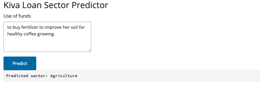
• train.py saves the fitted pipeline as a model pin using vetiver, alongside a separate pin for the held out test rows.
• deploy.py loads that pin and wraps it in a small FastAPI app via vetiver.VetiverAPI, exposing a /predict endpoint.
• app.py is a small Shiny for Python app with a text box for the loan description, which calls that local API and displays the predicted sector.
• app.py loads the model pin directly rather than calling the separate API, which keeps it deployable as a single, self-contained piece of content (handy on platforms that only publish one app at a time).

Here is the app in action, predicting the sector for a loan described as going toward fertilizer and coffee growing:

The Shiny app predicting “Agriculture” for a coffee farming loan description

Try the live predictor here, it’s deployed on Posit Connect Cloud and running the exact model described above.

Everything here runs locally aside from that live deployment, with pins standing in for a shared model store and vetiver standing in for a deployment layer. A real production setup at scale would likely also add authentication and monitoring, neither of which this small example attempts to solve.

It’s worth noting:

• This is not a credit risk or lending decision tool. It predicts a coarse sector label from text, nothing more.
• The three class taxonomy (Agriculture, Business, Personal) is a modeling shortcut, not an official Kiva category.
• The data covers one country (Uganda) and one lending platform (Kiva). There is no reason to expect this to generalize elsewhere without retraining.
• Two thousand rows is a small dataset. Treat the metrics above as a reasonable estimate for this specific slice of data, not a universal truth about the model’s quality.

Try it yourself

Play with the live predictor directly, no setup required.

The full code, including the extraction script, the tidying and training pipeline, the model card, and the Shiny app, is available in the kiva-ml repository on GitHub. The README walks through running each stage in order, from pulling fresh data to starting the local API and app.